Warning

Please note that the documentation you are currently viewing is for an older version of our technology. While it is still functional, we recommend upgrading to our latest and more efficient option to take advantage of all the improvements we’ve made. See DEX.

Integrate AIMMS with R

This article is part of a series of examples on how to connect AIMMS with models built in Python or R. We recommend you read both Connecting AIMMS with Data Science Models and How to connect AIMMS with Python before continuing.

In this article, we will show how to extend an AIMMS app with a R model that generates a Sankey diagram using the networkd3 package. The R model is exposed as a REST API using the Plumber package.

Example

We will use an implementation of the Blending problem, a classic application of linear programming. The objective is to find what composition of alloys should be blended together to make a final alloy with the required properties, minimizing cost. The model outputs the % composition of the final alloy - x% of Alloy A, y% of Alloy B, and so on. For example, using the provided data - a 60% Alloy B and 40% Alloy D mixture is the optimal way to create an alloy with 30% lead, 30% zinc, and 40% tin.

This breakdown can already be visualized in AIMMS WebUI using the treemap widget.

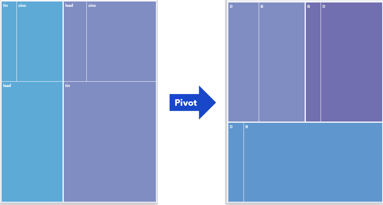
Fig. 16 Colors represent (a) alloys in the left image and (b) elements in the right image.

We can also visualize the same data in a Sankey diagram, which are typically used to visualize flows in multi-level networks. A sankey widget is not available in AIMMS and, instead of building a custom widget - one could use R (or Python) to generate the sankey diagram as an image. This example shows that in addition to running machine learning models, data processing and transformations, R / Python can also be used to generate visualizations for your AIMMS WebUI application.

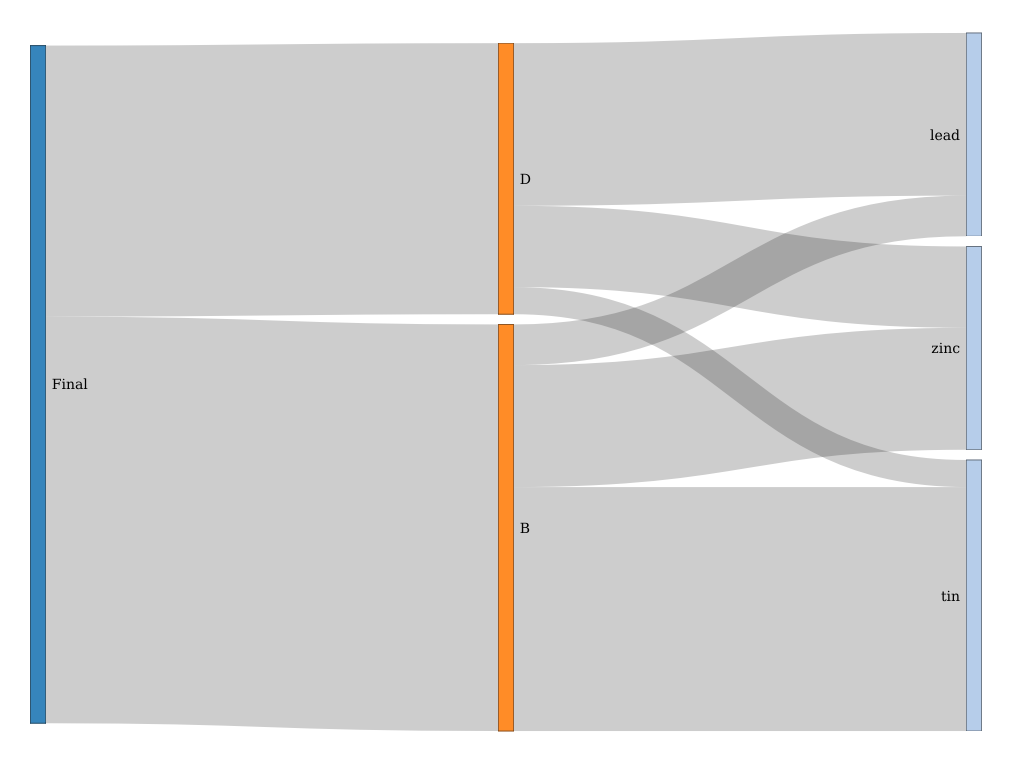
Fig. 17 View interactive version here

The example AIMMS and R projects we will refer to in this article can be downloaded from here. The download contains:

1. blendingModel: The AIMMS project folder which is an implementation of the Blending problem.

2. sankeyPlot: The R project which contains three .R scripts, a renv.lock file, and a test.json file. (more later)

3. Dockerfile: The docker file to containerize this R project.

Installing prerequisites

In addition to the prerequisites outlined in Development Tools, you will need to install the below for this example.

1. The example project is developed using AIMMS version 4.76.8, so we recommend you use at least that version. Download AIMMS Developer.

2. AIMMS HTTP Client Library: version 1.1.0.6 or above.

3. The R project in the example is developed in R 4.0.3.

4. renv package to install the dependencies captured in the renv.lock file. Read more.

   #install renv
   install.packages("renv")
   
   #restore packages
   renv::restore()
   

   Running the renv::restore() command once will install all the packages required for this code to run.

   Using the renv package is one way to use virtual environments while working with R - to share reproducible projects and to not change the packages already on your computer.

The R project

The R project folder sankeyPlot contains three .R scripts - model.R, api.R, and run_api.R.

model.R contains functions which take in a JSON file (in the required format) and return a sankey diagram in HTML and PNG formats, using the networkD3::sankeyNetwork function. sankeyNetwork requires two data frames as input - Links and Nodes, as shown below. The group attribute of Nodes is optional but is used to control the coloring of the nodes but it is required that the source and target values in Links, and node in Nodes are 0 indexed integers.

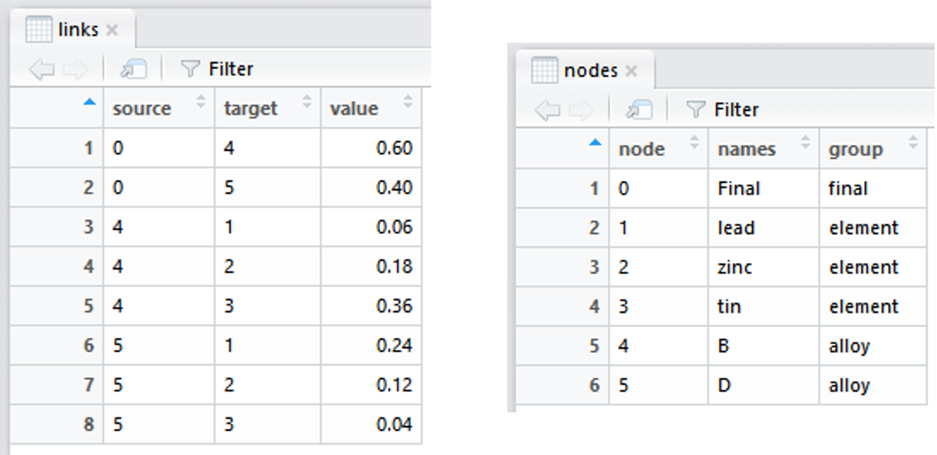
Fig. 18 Input data frames for the sankeyNetwork function.

A sample input file is provided in sankeyPlot/test.json. We use jsonlite::fromJSON() to import data from this file into R. So, running mySankey("test.json") will create the above sankey diagram (displayed in the Viewer pane of RStudio). hSankey("test.json") will return a .html file and iSankey("test.json") will return a .png file.

In api.R, we decorate different functions with special comments to expose them as API endpoints using the plumber package.

source("model.R")

#* Generate a sankey PNG
#* @get /sankey
#* @serializer contentType list(type='image/png')
sankey = function(req) {
  inFile <- req$postBody
  file <- iSankey(inFile)
  readBin(file,'raw',n = file.info(file)$size)
}

Lines 11 and 15 are required to specify that the response of this API is a PNG image file.

In this example, we have three APIs differentiated by the name following the #* @get comments in lines: 1, 10, 19. Here we define all three endpoints as GET but plumber also supports other API endpoints like POST, PUT, etc. Read more on plumber’s documentation.

1. / will return “hello world at _time” where _time is replaced by system time. A simple case to test the status of the API server.

2. /sankey will run the input JSON file through the iSankey function and return the output as a PNG image.

3. /sankeyHTML will run the input JSON file through the hSankey function and return the output as a HTML file.

In run_api.py, we use the plumber::plumb function to run (or plumb) the API server built in api.R. The port and host address are specified in line 4.

library(plumber)

r <- plumb("api.R")
r$run(port=8000, host="0.0.0.0")

Running locally

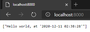
If you run the run_api.R file using source("run_api.R"), a local API server will be started. You can test this server by typing in the URL http://localhost:8000 in your browser.

We will use the Postman application to test the other two APIs which need a JSON body as input. Paste the contents of test.json in the Body attribute as shown below.

It will return the output in the bottom tab, as a PNG file or raw html code, depending on which API you call.

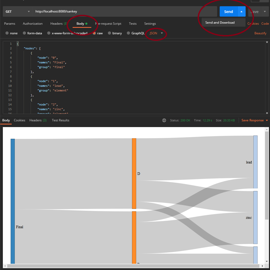
Make sure to set the attributes in the Body tab as raw, JSON. If you click on Send and Download instead of Send, Postman will let you download the response file.

The AIMMS project

The AIMMS project blendingModel has the input data and math model identifiers in declarations inputData and mathModel respectively.

Preparing data

v_alloyPurchased(i_alloy) contains the % composition of the final alloy. We need to use this identifier to prepare the input for the sankey API.

Section sankeyChart contains the declarations which hold the input data for the API. pr_createNodesFlows populates the set s_nodes and the identifiers indexed on this set - p_flows, sp_nodeNames, sp_nodeGroup.

Data I/O

prWriteJSON creates the input file as the R model expects, using the the mapping file blendingModel/mappings/outMap.xml. we export two dictionaries - nodes, and links and an array for the unit parameter up_percent.

<AimmsJSONMapping>
    <ObjectMapping>
        <ArrayMapping name="nodes">
            <ObjectMapping>
                <ValueMapping name="node" binds-to="i_node" />
                <ValueMapping name="names" maps-to="sp_nodeNames(i_node)"/>
                <ValueMapping name="group" maps-to="sp_nodeGroup(i_node)"/>
            </ObjectMapping>
        </ArrayMapping>
        <ArrayMapping name="links">
			<ObjectMapping>
				<ValueMapping name="source" binds-to="i_node" />
				<ValueMapping name="target" binds-to="j_node" />
				<ValueMapping name="value" maps-to="p_flows(i_node,j_node)" />
			</ObjectMapping>
		</ArrayMapping>
		<ValueMapping name="unit" maps-to="up_percent" />
    </ObjectMapping>
</AimmsJSONMapping>

As p_flows has two indices, it has two binds-to arguments (lines 12-13) whereas sp_nodeGroup and sp_nodeNames have the same one index, they get a single binds-to argument (line 5).

Calling the API

Now we simply use the HTTP library functions to make a GET call to the APIs created in the previous section. pr_healthCheck to check the status of the API and pr_iSankey to call the /sankey endpoint.

As the /sankey endpoint returns a PNG image, we do not need to read any data into AIMMS. Instead, we move the response file to the MainProject//WebUI//resources//images folder to be used by the Image widget, using FileMove.

pr_responseCheck;
if p_responseCode = 200 then
    sp_image := "sankey.png";
    FileMove(sp_inFile, sp_path, 1);
endif;

Deployment

Running the run_api.R script starts an API server on the local/development machine, on http://localhost:8000 or http://0.0.0.0/8000. These URLs will not be accessible to apps published on AIMMS PRO or AIMMS Cloud.

Hosting Plumber discusses some deployment options. As we did with the Flask APIs in How to connect AIMMS with Python, we will use Docker to deploy the Plumber APIs as well.

FROM rocker/rstudio:4.0.3

ENV RENV_VERSION 0.12.2
RUN apt-get update && apt-get install -y \
    libcurl4-openssl-dev \
    libsodium-dev
RUN R -e "install.packages('remotes', repos = c(CRAN = 'https://cloud.r-project.org'))"
RUN R -e "remotes::install_github('rstudio/renv@${RENV_VERSION}')"

COPY sankeyPlot sankeyPlot
WORKDIR sankeyPlot

RUN R -e 'renv::restore()'
RUN R -e "webshot::install_phantomjs(force = TRUE)"

EXPOSE 8000

ENTRYPOINT ["Rscript", "run_api.R"]

The image built using this dockerfile uses Rocker’s RStudio as a base. We use the RStudio version instead of the base rocker as some of the packages used in model.R need some dependencies that the base image does not have. Similarly, we install other dependencies like curl and libsodium in Line 4. Typically, a base docker image that satisfies all our needs can be found on sources like DockerHub or GitHub. If not, we will have to build our own custom dockerfile like in this case.

Lines 7 and 8 install R packages remotes and renv, only difference being in Line 8, we install a specific version of the package from the developer’s repository instead of from CRAN.

You can install all the required packages using either of these methods, but we use the renv::restore() as we did during development in Line 13.

Line 18 will run the run_api.R script when a container built on this image is started.

The below command line prompts will build a Docker image of the name imageName:latest and start a container. Building an image from this file takes up to 10 minutes, bulk of the time being spent in installing the R packages.

docker build --pull --rm -f "Dockerfile" -t imageName:latest "."

docker run -d -p 8000:8000 --name "containerName" imageName

This docker image can now be pushed to a container registry on a cloud service provider like AWS or Azure, from where the API server can be hosted.

Further reading

• Learn more about Plumber

• Serving images as response for Plumber API

• Serving HTML files as response for Plumber APIs