Modeling styles for using reference elements
This is a companion article to Modeling composite objects. That article and other companion articles show the advantages of the reference element approach. The modeling style used for the reference element approach in those articles is not the only possible modeling style for the reference element approach.
When there are multiple modeling styles, you want to select the best style for your application; hoping to avoid unnecessary changes to your application later on. To help you make a good choice regarding the modeling style for the reference element approach, this article compares a few modeling styles with respect to:
Modeling clarity.
Clarity of the model is crucial, as this will allow you to communicate the reality being modeled with the stakeholders more easily, and thereby gain their trust in the results of your application.
There is clarity in the declaration of the composite object itself, but more importantly, there is clarity in the use of composite objects in the application, for instance in the formulation of the constraints.
That is why the clarity will be evaluated by discussing the consequence of style when formulating a stock balance; similar to what is presented in Modeling composite objects
Modeling flexibility.
Flexibility in the application is important; how much effort is needed to update an application when a change in the structure is made? Regarding composite objects, a potential change is adding a component to the composite object - does it become necessary to edit every piece of source where the composite object is used?
In this article, a mode of transportation is added to the composite object arc. We will then discuss, for each modeling style, how much effort is needed for every reference to the composite object arc.
Execution efficiency.
The snappiness of the application when making small changes, the overall wait time when searching for a good solution; are in part determined by how the assignments and constraints are formulated.
In this article, a small model is used to measure the relative efficiency of the three styles. As a bonus, the component based approach is also part of these measurements.
The various modeling styles are presented in the next section, and then each of the evaluation criteria presented above is used to evaluate in a separate section. Finally, we present a brief summary and discussion.
The modeling styles
This article details three different modeling styles:
The multiple element parameter style; this is the style used in the main article and companion articles. Using this style, arcs are declared as follows:
 1Set s_arcIds {
 2    Index: i_arc;
 3}
 4ElementParameter ep_arcNodeFrom {
 5    IndexDomain: i_arc;
 6    Range: s_nodes;
 7    Comment: "Return the node from which the arc 'i_arc' flows""}
 8ElementParameter ep_arcNodeTo {
 9    IndexDomain: i_arc;
10    Range: s_nodes;
11    Comment: "Return the node to which the arc 'i_arc' flows""}
There is an element parameter for every component in the composite object.
The multiple binary parameter style; this is a small variation of the element parameter style. Using this style, arcs are declared as follows:
 1Set s_arcIds {
 2    Index: i_arc;
 3}
 4Parameter bp_arcIsFromNode {
 5    IndexDomain: (i_arc,i_node);
 6    Range: binary;
 7    Comment: "The arc 'i_arc' flows out of node 'i_node'""}
 8Parameter bp_arcIsToNode {
 9    IndexDomain: (i_arc,i_node);
10    Range: binary;
11    Comment: "The arc 'i_arc' flows towards node 'i_node'""}
There is a two-dimensional binary parameter for every component in the composite object.
The single encompassing binary parameter style; this style is similar to relational tables. Using this style, arcs are declared as follows:
1Set s_arcIds {
2    Index: i_arc;
3}
4Parameter bp_arcRelation {
5    IndexDomain: (i_arc,i_fromNode,i_toNode);
6    Range: binary;
7    Comment: "The arc 'i_arc' flows out of 'i_fromNode' towards 'i_toNode'""}
There is one entry in this parameter for every arc. The binary parameter has an index for the arc and for every component in the arc. It is reminiscent of the component based approach; as it can be viewed as the component based approach extended with a reference element.
Recap running example
This article continues the running example presented in Modeling composite objects. In particular, the following declarations will be used:
Sets
We start with a set of discrete time periods and a set of locations.
1Set s_timePeriods {
2    SubsetOf: Integers;
3    Index: i_tp;
4}
5Set s_nodes {
6    Index: i_node, i_nodeFrom, i_nodeTo;
7}
Parameters and variables
Data and variables are defined over these sets as usual, for instance,to track stock over time there is an initial stock and a variable modeling stock:
1Parameter p_initialStock {
2    IndexDomain: i_node;
3    Comment: "Stock at the beginning of the first period""}
4Variable v_stock {
5    IndexDomain: (i_tp,i_node);
6    Range: nonnegative;
7    Comment: "Stock at end of period i_tp""}
Set with reference elements
Arcs can be enumerated by numbering them and putting these numbers in a separate set:
1Set s_arcIds {
2    Index: i_arc;
3}
Variable declared over set with reference elements
1Variable v_flow {
2    IndexDomain: (i_tp,i_arc);
3    Range: nonnegative;
4}
Modeling clarity
In this section, we evaluate the formulation of a stock balance per node, where materials are flowing in to and out of that node, production increases stock, and demand decreases stock.
Clarity: The multiple element parameter style
The stock balance is the same as presented in Modeling composite objects.
 1Constraint c_stockBalance {
 2    IndexDomain: (i_tp,i_node);
 3    Definition: {
 4        v_stock(i_tp,i_node) ! Stock at end of period i_tp
 5            =
 6            if i_tp = first( s_timePeriods ) then
 7                p_initialStock(i_node)
 8            else
 9                v_stock( i_tp - 1, i_node ) ! Stock at end of previous period
10            endif
11            +
12            sum( i_arc | ep_arcNodeTo(i_arc) = i_node,
13                v_flow( i_tp, i_arc ) ) ! Total flow into i_node during period i_tp
14            -
15            sum( i_arc | ep_arcNodefrom(i_arc) = i_node,
16                v_flow( i_tp, i_arc ) ) ! Total flow out of i_node during period i_tp
17            +
18            v_production(i_tp, i_node)
19            -
20            p_demand(i_tp, i_node)
21    }
22}
Lines 12 and 15 are emphasized, as here the composite structure of arcs plays a role.
On line 12, the condition ep_arcNodeTo(i_arc) = i_node clearly states that a flow to i_node is considered an inflow for i_node.
Clarity: The multiple binary parameter style
The same stock balance, but now using the binary parameter style:
 1Constraint c_stockBalance {
 2    IndexDomain: (i_tp,i_node);
 3    Definition: {
 4        v_stock(i_tp,i_node) ! Stock at end of period i_tp
 5            =
 6            if i_tp = first( s_timePeriods ) then
 7                p_initialStock(i_node)
 8            else
 9                v_stock( i_tp - 1, i_node ) ! Stock at end of previous period
10            endif
11            +
12            sum( i_arc | bp_arcIsToNode(i_arc,i_node),
13                v_flow( i_tp, i_arc ) ) ! Total flow into i_node during period i_tp
14            -
15            sum( i_arc | bp_arcIsFromNode(i_arc,i_node),
16                v_flow( i_tp, i_arc ) ) ! Total flow out of i_node during period i_tp
17            +
18            v_production(i_tp, i_node)
19            -
20            p_demand(i_tp, i_node)
21    }
22}
On line 12, the condition bp_arcIsToNode(i_arc,i_node) clearly represents the same condition as the condition ep_arcNodeTo(i_arc) = i_node above, but comes across as a translation towards a more efficient representation for the computer.
Clarity: The single encompassing binary parameter style
 1Constraint c_stockBalance {
 2    IndexDomain: (i_tp,i_node);
 3    Definition: {
 4        v_stock(i_tp,i_node) ! Stock at end of period i_tp
 5            =
 6            if i_tp = first( s_timePeriods ) then
 7                p_initialStock(i_node)
 8            else
 9                v_stock( i_tp - 1, i_node ) ! Stock at end of previous period
10            endif
11            +
12            sum( (i_arc,i_fromNode) | bp_arcRelation(i_arc,i_fromNode,i_node),
13                v_flow( i_tp, i_arc ) ) ! Total flow into i_node during period i_tp
14            -
15            sum( (i_arc,i_toNode) | bp_arcRelation(i_arc,i_node,i_toNode),
16                v_flow( i_tp, i_arc ) ) ! Total flow out of i_node during period i_tp
17            +
18            v_production(i_tp, i_node)
19            -
20            p_demand(i_tp, i_node)
21    }
22}
On line 12, the condition becomes: bp_arcRelation(i_arc,i_fromNode,i_node) which is slightly more detail as in the previous style. More importantly, however, the summation operator has an extra index, which makes understanding the reason behind the condition less easy.
Modeling flexibility
Flexibility is tested here by changing the structure of an arc. Each arc gets an additional mode of transport.
1Set s_transportModes {
2    Index: i_tMode;
3}
Flexibility: The multiple element parameter style
The arcs are extended with an additional element parameter, as follows:
1ElementParameter ep_arcTransportMode {
2    IndexDomain: i_arc;
3    Range: s_transportModes;
4    comment: "Return the mode of transport used to flow over the arc 'i_arc'";
5}
Regarding the stock balance; the formulation stays the same.
Note, however, if different modes of transport are allowed between two nodes, there are now multiple arcs between those nodes, thereby increasing the number of inflow arcs and the number of outflow arcs for a particular node.
Flexibility: The multiple binary parameter style
The arcs are extended with an additional binary parameter, as follows:
1Parameter bp_arcUsesTransportMode {
2    IndexDomain: (i_arc,i_tMode);
3    Range: binary;
4    comment: "The arc 'i_arc' uses transport mode 'i_tMode'";
5}
Regarding the stock balance; the formulation stays the same.
A similar note regarding additional inflow and outflow arcs for a particular node applies here as well.
Flexibility: The single encompassing binary parameter style
1Parameter bp_arcRelation {
2    IndexDomain: (i_arc,i_fromNode,i_toNode,i_tMode);
3    Range: binary;
4    comment: "The arc 'i_arc' flows out of 'i_fromNode' towards 'i_toNode' using transport mode 'i_tMode'";
5}
 1Constraint c_stockBalance {
 2    IndexDomain: (i_tp,i_node);
 3    Definition: {
 4        v_stock(i_tp,i_node) ! Stock at end of period i_tp
 5            =
 6            if i_tp = first( s_timePeriods ) then
 7                p_initialStock(i_node)
 8            else
 9                v_stock( i_tp - 1, i_node ) ! Stock at end of previous period
10            endif
11            +
12            sum( (i_arc,i_fromNode,i_tMode) | bp_arcRelation(i_arc,i_fromNode,i_node,i_tMode),
13                v_flow( i_tp, i_arc ) ) ! Total flow into i_node during period i_tp
14            -
15            sum( (i_arc,i_toNode,i_tMode) | bp_arcRelation(i_arc,i_node,i_toNode,i_tMode),
16                v_flow( i_tp, i_arc ) ) ! Total flow out of i_node during period i_tp
17            +
18            v_production(i_tp, i_node)
19            -
20            p_demand(i_tp, i_node)
21    }
22}
As bp_arcRelation(i_arc,i_fromNode,i_node,i_tMode) has an additional index, the condition needs to be adapted and the summation index list extended, further obfuscating the interpretation of the condition.
Execution efficiency
When comparing execution efficiency, doing an actual test is a good starting point. The three styles are tested regarding execution efficiency and also compared to the component based approach. To make the comparison meaningful, the running example is slightly modified:
A set of product groups with index
i_pgis added,The flow is modeled as a parameter
p_flow(i_tp, i_pg, i_arc)with a flow of 1 for every element.The index
i_tp(time periods) varies over a set with 200 elements, the indexi_pg(product groups) varies over a set of 100 elements, the indexi_nodevaries over a set with 1000 elements, and the indexi_arcvaries over a set with 5000 elements.
This leads to the following comparison of execution times:
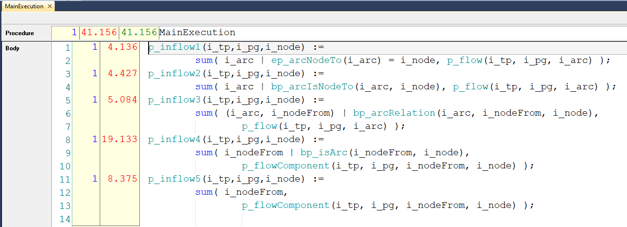
where
The
p_inflow1is computed using the reference element approach with the multiple element parameter styleThe
p_inflow2is computed using the reference element approach with the multiple binary parameter styleThe
p_inflow3is computed using the reference element approach with the single encompassing binary parameter styleThe
p_inflow4is computed using the component approach and selecting from nodes in the summation operator.The
p_inflow5is computed using the component approach, and leaving the selection of the from nodes to the index domain condition in the declaration ofp_flowComponent, thus avoiding a duplicate selection of from nodes.
In this test, the reference element based approach (p_inflow1, p_inflow2, and p_inflow3) performs significantly superior to the component based approach (p_inflow4, p_inflow5).
In addition, within the reference element based approach, the formulation using multiple element parameter style is the fastest, but the timings of the three styles are close.
To play around with this example, you can download the AIMMS 4.82 project here.
Summary and discussion
To summarize:
From the tests on the reference element approach presented in this article, the style: The multiple element parameter style clearly performs best overall.
To discuss:
At the time of writing this article, the reference element based approach to composite objects is not in widespread use; thus the tests presented above are admittedly artificial. The author is looking forward to applications whereby the reference element based approach is actually used in practice, such that a comparison of styles, and perhaps also a comparison to the component based approach can be made that is closer to actual modeling practice.